Introduction
A major thesis in global warming theory has been that higher air temperatures will cause increased evaporation leading to even more greenhouse warming from the added water. This thesis seems to rest largely on the observation that the equilibrium vapor pressure of water increases almost exponentially with temperature, combined with classical evaporation theory which assumes that evaporation is driven by undersaturation. Though the view seems to be shifting, for decades climate science has asserted that water vapor is “a feedback not a forcing”. Results which lead to this conclusion are based on models -apparently radiative convective equilibrium with fixed relative humidity- which assume that warmer air temperatures alone can increase water vapor evaporation (Schmidt 2005) , (SOD 2017) . As (McKitrick 2021) reminds us, global warming theory is still not rigorously proven.
Column Water as a Function of Sea Surface Temperature
It is possible to treat the relation between sea surface temperature and column water as a statistical matter. With the near magic of satellite observations we can determine the extent to which atmospheric water vapor is related to ocean surface temperature. The NASA site https://neo.sci.gsfc.nasa.gov/ provides weekly averaged data on clear sky average column water (CW) and satellite based sea surface temperature(SST) . It is important to emphasize that these satellite measures of surface temperature can only take place on relatively clear days, and that diurnal cycles of precipitation are not explicitly part of the measurement. Satellite derived temperatures are accurately described as skin sea surface temperatures, SSST, which usually differ from thermometric temperatures. For the remainder of this note we will use the SST and SSST interchangeably. A good comparison of various skin temperatures is found in (Webster et al. 1996) which is a veritable primer on what happens in the tropical oceans.
The starting point is two files averaged for a particular week, one with CW the other with SST. The global data are spherical coordinate arrays (720,360), 1/2 degree longitude(index i) by latitude (index j). We can construct a plot of CW on the Y axis versus SST on the X axis, shown in Figs. 1N and S .
Using the Clausius Clapeyron water vapor pressure equation for temperature T in Celsius we can produce a non dimensional fitting function Cz(T) approximated with the exponential term of the Tetens vapor pressure equation.
Cz(T) = CC(T)/CC(0)= exp( (17.67*T)(T + 243.5)) Eq. 1
We can define the fitting function of temperature CF(T) as Wc * Cz( SST (i,j)) where Wc is a factor which changes by week and hemisphere. The error of the fit to be least squares minimized by variation of Wc for each hemispheric data set will be
e(i,j) = CF( SST(I,j) ) – CW(I,j) = Wc * Cz( SST(I,j) ) – Cw( SST(I,j)) Eq. 2
The factor Wc is the least squares fitted value of column water at zero C. WC has dimensions of cm of water. Column water may vary with both season and hemisphere , so there are 52 weeks and 2 hemispheres to span a year. Such a plot is shown in Fig 1. See (Note 1) for some file names. The evaluation of water vapor as a function of SST is not new. There are many such studies, of which an early one is (Stephens 1990). A more recent one is (Kanemaru and Masunaga 2012).
It is reasonable to ask how well the fitted CF(T) matches the data. One measure of the extent to which a fitted curve matches ratio scaled data with a zero reference is the ratio of the standard deviation of the error of the fit to deviation of the original data, known as relative standard deviation, RSD. RSD is useful for evaluating fits when the data spans wide ranges as does the vapor pressure of water across the planet.
Treating each temperature from a set of SST(I,j) as an integer IT = (e(I,j)+.5) there are multiple observations. RSD(IT) is the standard deviation of all e(i,j) at temperature IT divided by the root mean square average of all CW(I,j) at temperature IT and shown in Fig. 1. The average of all the RSD(IT) at each data set, weighted by the average cosine of latitude is reported in a table as the “unresolved variability fraction.” The word variability here is distinct from variance. An approximation to the variance ratio of errors to data would be the square of this variability ratio.
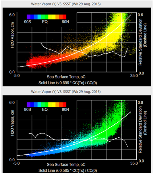
Figures 1 N and S: Column Water Vapor as function of Ocean Surface Temperature in Northern and Southern Hemispheres. Colors based on latitude range from red at north pole to blue at south pole. The curved solid white line is proportional to the Clausius-Clapeyron (CC) equation for vapor pressure and scaled to fit the water vapor data. The scaled curve, WC CC(SST)/CC(0) has the dimensions of centimeters of water vapor. The colored pixels, 1/2 deg.squared, of which there are many more at the equator, do not indicate the frequency of data points which is usually about 40,000 jointly available out of about 100,000 ocean and clear sky observations. For 1N WC is 0.699 and for 1S 0.585. The dotted curve “Relative Standard Deviation” is the ratio of the standard deviation of the e(I,j) at temperature IT to the standard deviation of SST(I,j) at temperature IT which we are calling here “unresolved variability”.
In the following table WC is seen to be different for different hemispheres and for different times of the year. The entries in the table are cherry picked in that not all weeks show such docile fits, particularly those at the change of seasons. Several of those listed show clear splits where some of the WV data is consistent with one WC while the rest are with one quite different. See note (WVsplit) for an example. The data points cooler than the split do not significantly change the weighted average unresolved variability. Wc is the fitted value of column water at zero C. To the extent that Equation 1 fails to fit ocean water Wc will be in error and the unresolved variability increased.
Table of parameters Wc from a selected sampling of weekly fits of water vapor to SST
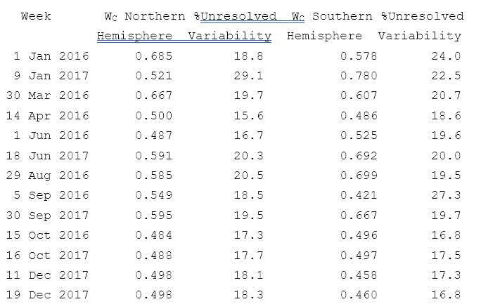
The unresolved variability fraction listed in the table is an area weighted average of the points plotted on the curve. This places far more weight on the points nearer to the equator, as does the least squares fit.
A dramatic observation of the various fitted CW versus SST is that the fractional variability attributable to the fitted curve often accounts for 80% of the total variability of the data for a particular hemisphere and week of year. This fit spans many km of open ocean and temperatures ranging from near 0 to 34OC. Wc is relatively constant, from 0.42 to 0.8 cm for several dozen data sets for several years of data while the column water values range from 0.5 to 5.
What is different here from many previous studies that usually show high levels of variability of the CC functional dependence? First, this analysis treats all the variation associated with planetary geography and weather patterns across each hemisphere as a source of variation rather than the use of anomalies from an average base. Second, satellite based SST is used rather than thermometric temperature. Third, weekly averages are used rather than much longer time averages. This interval is useful for extracting the 3-5 day SST-cloud cycle noted by (Webster et al. 1996 ). Fourth, separating the hemispheres helps to isolate the seasonal variation. Fifth, clear sky measurements avoid the complications of cloud and condensation.
Discussion
The high variability contribution to column water from CC(SST) suggests that on average column water over oceans is largely governed by the measured local SST though likely modulated by wind and surface processes including biological. If we view Eq. 1 as a process with SST as the single input and CW as an output, statistics alone cannot separate noise in the measurements from errors of the process. Clearly the evolution of CW takes time, which is not nominally a parameter in the statistical Eq. 1. The unresolved variability fraction of about 20% is a 4:1 signal to noise ratio or 12 db. This is not high but allows recognition by most standards. Even if all error is attributed to the process, it still appears that about 80% of the variability in CW arises from variability in SST. Given that the number of data points for each value in Table 1 is on the order of 20,000 subdividing the hemisphere might further reduce the unresolved variability with negligible loss in the number of degrees of freedom.
The results here are not consistent with models which suggest that atmospheric forcing alone is sufficient to drive evaporation to increasingly higher levels. These results suggest that most of the variation must be manifested as SST change. The kinetics of evaporation implemented in most climate models up to and including CMIP5, are apparently derived from early enthalpy transfer studies, of which one is (Lui et al. 1979). The bulk formula is discussed in the Isaac Held’s excellent blog. From (Held #47)
” —– evaporation over the oceans can be approximated by the “bulk formula”

Eq. 3
Here ![]() and
and ![]() are the saturation humidities at the ocean surface and reference level temperatures respectively, and are the relative humidity and wind speed at this reference level, the atmospheric density and a non-dimensional constant. A lot of physics and a lot of empirical evidence has been stuffed into the constant , guided by what is affectionately known as Monin-Obukhov similarity theory. (All global climate models compute surface fluxes using Monin-Obukhov scaling as the starting point.) depends on the height of the reference level, some properties of the surface (specifically surface “roughnesses”), and the gravitational stability of the atmosphere near the surface, which in turn is strongly coupled to the air-sea temperature difference. If we ignore the air sea temperature difference as well as changes in wind speed and , then we just have
are the saturation humidities at the ocean surface and reference level temperatures respectively, and are the relative humidity and wind speed at this reference level, the atmospheric density and a non-dimensional constant. A lot of physics and a lot of empirical evidence has been stuffed into the constant , guided by what is affectionately known as Monin-Obukhov similarity theory. (All global climate models compute surface fluxes using Monin-Obukhov scaling as the starting point.) depends on the height of the reference level, some properties of the surface (specifically surface “roughnesses”), and the gravitational stability of the atmosphere near the surface, which in turn is strongly coupled to the air-sea temperature difference. If we ignore the air sea temperature difference as well as changes in wind speed and , then we just have

. “
In the bulk formula, Eq. 3, the temperatures TO and TA specify gas phase humidities at the air-water interface representing the rates at which molecules leave and arrive at the surface. An implementation problem with the bulk formula is that much of the volume of gas above the surface is more or less at equilibrium with the surface, so can be correlated with it. Extracting temperatures to make the bulk formula consistent with actual measurements is the subject of multiple papers and several empirical parameters. (Clayson et al. 1996) provides a view of the complexity.
A theoretical problem with Eq. 3 is that the function qS(To) is usually taken to be the CC equation, the derivation of which assumes equilibrium between the liquid and vapor phases. If the phases are not in equilibrium the CC equation may not give the correct pressures, and if they were in equilibrium there would be no net evaporation. The use of equilibrium theories can work so long as the underlying molecular distributions are not severely perturbed. Observed evaporation rates are far from equilibrium and neither Eq. 3 nor (Clayson et al. 1996) seem able to incorporate the work of (Ward et. al. 2001) and (Badam et al. 2007) on the non-Maxwellian molecular distributions of evaporation (Almenas 2015) which might require significant nonlinear adjustments.
To circumvent deficiencies in theory, empirical parameters such as the constant C in Eq. 3 are adjusted to match experimental data. To complicate matters further, many of the older general circulation models operate with fixed SST and so are not energetically consistent. Parameters in such models adjusted to match historical data may not be useful for predictions under changed conditions.
If Eq. 3 does not work, how then could Eq. 1? The clear sky average value of CW and SST over a multiday period is the result of diurnal cycles of evaporation, convection, condensation, heating and cooling. In the midst of all this activity there will be some computable average value of temperature. It is not impossible that the average temperature resulting from these processes should be near to the observed average SST. The significance of Eq 1 for this study is that it has statistical importance, not so much scientific.
The statistical results here suggest that nature has done the job of netting the diurnal variable terms, and adjusted the SST to conform to the relevant conditions so that observed evaporation is dominated by qS(SST). The residual 20% variation may be due convection and relative humidity effects term. This parallels arguments by (Matthews and Matthews 2014) who say that evaporation is not controlled by the bulk formula parameters but by surface temperature.
Looking Fig 1, one might be tempted to assert the possibility of CO2 radiatively forcing SST. A problem with this argument is that the radiative properties of CO2 at sea level are overwhelmed by the water vapor radiative properties at any CW much above 1 cm of water (Wong and Minnett 2018) and (Note 2) using MODTRAN. CO2 might have measurable effect in the polar oceans where CW can get as low as 1/2 cm, from Fig. 1 within 30 degrees of the poles. Cloud thermal radiation can dominate CO2 radiation for all values of CW. Given the percentage of time the sky is clear rather than cloudy, and the relative amount of radiative forcing under both conditions, the time averaged activity of CO2 seems small.
From Fig. 1 the CC relation is beginning to fail at higher temperatures but the relative number of clear sky data points is going rapidly to zero as if some sort of threshold has been reached at column water around 4 cm. and temperatures around 27OC. It is likely not a coincidence that the latter is the temperature associated with cyclogenesis. These are also the conditions where condensation is increasingly likely to be water droplets rather than ice. See (Romps 2017).
Summary
In summary, approximately three quarters of the variability of clear sky column water above the planetary oceans is explained by a scaled version of the Clausius-Clapeyron equation for the vapor pressure using satellite determined sea surface temperature. To the extent these arguments are valid, water vapor production cannot be accurately modeled as either a feedback or a result of CO2 forcing as suggested by (Schmidt 2005) .
Similarly, the majority of any water vapor feedback must occur through interaction with the surface waters. This mechanism could severely restrict both the magnitude and proximity in time of any catastrophic warming since oceans warm much more slowly than air from atmospheric forcing.
To quote from (Hoyos and Webster 2011) “A key to understanding the evolution of Earth’s climate is deciphering the relationship between tropical convection and the magnitude and gradients of the local sea-surface temperature.” Such work is underway (Tomassini 2020) .
References and Notes
(Almenas 2015 ) K. Almenas, Evaporation/Condensation of Water: Unresolved Issues
(Badam et al. 2007) Experimental and theoretical investigations on interfacial temperature jumps during evaporation
V. K. Badam, V. Kumar, F. Durst, K. Danov
Experimental Thermal and Fluid Science, V 32, #1, October 2007, pp 276-292
https://doi.org/10.1016/j.expthermflusci.2007.04.006
(Clayson et al.) Determination of surface turbulent fluxes for the Tropical Ocean-Global Atmosphere Coupled Ocean-Atmosphere Response Experiments: Comparison of satellite retrievals and in situ measurements
C. A. Clayson, J. A. Curry
J. Geophysical Research V. 101 #2, p. 28,515-28,528 Dec. 15, 1996
(Held #47) https://www.gfdl.noaa.gov/blog_held/47-relative-humidity-over-the-oceans
(Hoyos and Webster 2011) Evolution and modulation of tropical heating from the last glacial maximum through the twenty-first century
Carlos D. Hoyos , Peter J. Webster
Clim. Dyn. (2012) 38:1501—1519
DOI 10.1007/s00382-011-1181-3
(Kanemaru and Masunga 2012) A Satellite Study of the Relationship between Sea Surface Temperature and Column Water Vapor over Tropical and Subtropical Oceans
Kaya Kanemaru and Hirohiko Masunaga
J. Climate, 15 Jun 2013 , pp 4204-4218
DOI: https://doi.org/10.1175/JCLI-D-12-00307.1
(Liu et al. 1979 ) Bulk Parameterization of Air-Sea Exchanges of Heat and Water Vapor Including the Molecular Constraints at the Interface
W. Timothy Liu, Kristina Katsaros, Joost Businger
J. Atmospheric Sciences, Volume 36: Issue 9
https://doi.org/10.1175/1520-0469(1979)0362.0.CO;2
(Matthews and Matthews 2014) In situ measurement shows ocean boundary layer physical processes control catastrophic global warming.
Matthews, J. B., & Matthews, J. B. R. (2014).
Journal of Advances in Physics, 5(1), 681–704.
https://rajpub.com/index.php/jap/article/view/1625
(McKitrick 2021) https://judithcurry.com/2021/08/18/the-ipccs-attribution-methodology-is-fundamentally-flawed/#more-27816
(Note 1) The data used in figure 1 are from https://neo.gsfc.nasa.gov/ files MYD28W_2016-03-29_rgb_720x360.CSV for SST and MYDAL2_E_SKY_WV_2016-03-30_rgb_720x360.CSV for WV.
(Note 2) U. Chicago MODTRAN
https://climatemodels.uchicago.edu/modtran/
Table of selected MODRAN results for Sea Level Down Welling Radiation in watts per sq. meter.
Parameters other than defaults used were Locality: Tropical Atmosphere, Altitude: 0, Looking up
Water Vapor Scale 0.5 1 2 3 4
No Clouds
CO2 400 ppm 328.13 369.26 423.90 442.42 447.76
CO2 800 ppm 331.58 371.14 424.21 ” “
Stratus cloud base (.33KM, Top 1.0km)
CO2 400 ppm 449.64 449.96 450.90 451.53 451.84
(Rahimi and Ward 2005) Kinetics of Evaporation: Statistical Rate Theory approach
Payam Rahimi, Charles Ward
International Journal of Thermodynamics, Vol 8 (No1) , pp 1-14, March 2005
(Romps 2017) Exact Expression for the Lifting Condensation Level
David M. Romps J. Atm Sciences v74:12 01 Dec. 2017
https://doi.org/10.1175/JAS-D-17-0102.1
(Schmidt 2005) https://www.realclimate.org/index.php/archives/2005/04/water-vapour-feedback-or-forcing/#more-142
“To first approximation, the water vapour adjusts to maintain constant relative humidity. It’s important to point out that this is a result of the models, not a built-in assumption. Since approximately constant relative humidity implies an increase in specific humidity for an increase in air temperatures, the total amount of water vapour will increase adding to the greenhouse trapping of long-wave radiation. This is the famed ‘water vapour feedback’.”
(Small et al. 2019) Air–Sea Turbulent Heat Fluxes in Climate Models and Observational Analyses: What Drives Their Variability?
R Justin Small, Frank O. Bryan, Stuart P Bishop, Robert Tomas
Journal of Climate, Vol 32, issue 8 15 Apr 2019 p.2397–2421
https://doi.org/10.1175/JCLI-D-18-0576.1
(SOD 2017)
(Stephens 1990) On the Relationship between Water Vapor over the Oceans and Sea Surface Temperature
Graeme L. Stephens J. Climate, 1 June 1990, pp 634-645
https://doi.org/10.1175/1520-0442(1990)0032.0.CO;2
(Tomassini 2020) The Interaction between Moist Convection and the Atmospheric Circulation in the Tropics
Lorenzo Tomassini
BAMS 27 Aug 2020 E1378–E1396
DOI: https://doi.org/10.1175/BAMS-D-19-0180.1
(Ward et al. 2001)Analysis of the Interfacial conditions during evaporation or condensation of water
Ward C. A., D. Stanga
Physical Rev. E, Vol. 64, pp. 05159091– 05159099. (2001)
https://doi.org/10.1103/PhysRevE.64.051509
(Webster et al. 1996 ) Clouds, Radiation, and the Diurnal Cycle of Sea Surface Temperature in the Tropical Western Pacific Peter J. Webster, Carol Anne Clayson, and Judith A. Curry J. Climate. 01 Aug 1996 https://doi.org/10.1175/1520-0442(1996)009<1712:CRATDC>2.0.CO;2
(Wong and Minnett 2018) The Response of the Ocean Thermal Skin Layer to Variations in Incident Infrared Radiation Elizabeth W. Wong, Peter J. Minnett JGR Oceans Volume 123, Issue 4, April 2018, pp. 2475-2493

Critical comments accepted.